


Spark Streaming part 4: clustering with Spark MLlib

Jun 27, 2019
Never miss our publications about Open Source, big data and distributed systems, low frequency of one email every two months.
Spark MLlib is an Apache’s Spark library offering scalable implementations of various supervised and unsupervised Machine Learning algorithms. Thus, Spark framework can serve as a platform for developing Machine Learning systems. An ML model developed with Spark MLlib can be combined with a low-latency streaming pipeline created with Spark Structured Streaming. The K-means clustering algorithm will be incorporated into the data pipeline developed in the previous articles of the series.
This is the final article of a four-part series:
- In the first part, a data pipeline with a Spark Structured Streaming application is built.
- The second part concerns the migration of the pipeline to a Hadoop cluster.
- In the third part, the PySpark application was ported to Scala Spark and unit tested.
- The fourth and last part enriches the data pipeline with a Machine Learning clustering algorithm.
In order to enrich the existing pipeline with Machine Learning algorithm, the following phases will be covered:
- Data engineering to prepare ML input
- ML model development
- Integration of the ML model within the streaming data pipeline
A Spark MLlib pipeline is trained on historic data in batch mode. Then, the resulting model will be used in a separate Spark streaming application. The computations of the clusters are supposed to be periodically relaunched to update the ML model.
The project’s source code can be found in the adaltas/spark-mllib-streaming GitHub repository. This project extends the Scala Spark application from spark-streaming-scala repository with a Machine Learning k-means clustering algorithm.
Use case for clustering
The use case central to the whole series is about NYC Taxi drivers wanting to get higher tips. The question that we sought to answer in the previous parts of the series was:
What Manhattan neighborhood should a Taxi driver choose to get a high tip?
This question imposes a spatial granularity determined by Manhattan’s neighborhoods. A Taxi driver can be informed only of a neighborhood with an elevated tip, without a more precise location. Following this question, the solution developed previously was based on the administrative division of Manhattan.
A finer granularity than neighborhoods would improve the usefulness of the service and address the use case better. The question can be generalized:
Which Manhattan area should a Taxi driver choose to get a high tip?
An area could be any zone of arbitrary size. Instead of partitioning Manhattan into neighborhoods, we will search for small zones with elevated tip. A Machine Learning k-means algorithm will be leveraged to obtain areas of interest. Each such an area is a cluster of Taxi rides with elevated tips. A cluster of Taxi rides will be later on called cluster.
Notice that a cluster has two distinctive meanings. A cluster in the cluster analysis, e.g. cluster of Taxi rides, and a cluster in distributed systems, as a Hadoop cluster. Both terms are relevant to the article and the type of cluster meant should be clear from the context.
Clustering is an unsupervised learning task of grouping similar objects. Such tasks can’t be evaluated easily, because the ground truth isn’t available and pre-existing output labels don’t exist. Taxi rides don’t belong naturally to any particular “solution cluster”. The partitioning obtained with clustering could be good or bad, depending on the use case and the interpretation. The choice of the number of clusters k, which has the biggest impact on the obtained clusters, is largely subjective.
Getting Taxi data
The used dataset is the Taxi data slightly modified for the Apache Flink Training. It’s a small, 100MB dataset obtained from the original NYC Taxi Rides data.
If you have a Hadoop cluster and followed the second part of the series, the raw dataset is already available in directories “/tmp/datalake/RidesRaw” and “/tmp/datalake/FaresRaw” on HDFS. In this case, use the data from those locations and skip the rest of this section.
You can follow this part of the series without a Hadoop cluster. Scala Spark application below creates the needed raw dataset on a local filesystem. Data is stored in the Parquet file format and follows the same data partitioning as in previous parts of the series.
Start by downloading the Flink’s compressed datasets: nycTaxiRides.gz and nycTaxiFares.gz.
# from project's directory
curl -s https://training.ververica.com/trainingData/nycTaxiRides.gz -o nycTaxiRides.gz
curl -s https://training.ververica.com/trainingData/nycTaxiFares.gz -o nycTaxiFares.gz
Then, create a Scala file: “src/main/scala/com/adaltas/taxistreaming/DataLoader.scala” belonging to the com.adaltas.taxistreaming package.
package com.adaltas.taxistreaming

import org.apache.spark.sql.functions.{col, dayofmonth, month, year}
import org.apache.spark.sql.types._
import org.apache.spark.sql.{DataFrame, SparkSession}

object DataLoader {

  def main(args: Array[String]): Unit = {

    val spark = SparkSession.builder
      .appName("Local fs data writer")
      .master("local")
      .getOrCreate()

    val taxiRidesSchema = StructType(Array(
      StructField("rideId", LongType), StructField("isStart", StringType),
      StructField("endTime", TimestampType), StructField("startTime", TimestampType),
      StructField("startLon", FloatType), StructField("startLat", FloatType),
      StructField("endLon", FloatType), StructField("endLat", FloatType),
      StructField("passengerCnt", ShortType), StructField("taxiId", LongType),
      StructField("driverId", LongType)))

    val taxiFaresSchema = StructType(Seq(
      StructField("rideId", LongType), StructField("taxiId", LongType),
      StructField("driverId", LongType), StructField("startTime", TimestampType),
      StructField("paymentType", StringType), StructField("tip", FloatType),
      StructField("tolls", FloatType), StructField("totalFare", FloatType)))

    var dfRides = spark.read
      .option("header", false)
      .option("inferSchema", false)
      .schema(taxiRidesSchema)
      .csv("nycTaxiRides.gz")

    var dfFares = spark.read
      .option("header", false)
      .option("inferSchema", false)
      .schema(taxiFaresSchema)
      .csv("nycTaxiFares.gz")

    dfRides
      .withColumn("year", year(col("startTime")))
      .withColumn("month", month(col("startTime")))
      .withColumn("day", dayofmonth(col("startTime")))
      .write
      .format("parquet")
      .partitionBy("year", "month", "day")
      .save("datalake/RidesRaw")

    dfFares
      .withColumn("year", year(col("startTime")))
      .withColumn("month", month(col("startTime")))
      .withColumn("day", dayofmonth(col("startTime")))
      .write
      .format("parquet")
      .partitionBy("year", "month", "day")
      .save("datalake/FaresRaw")

    spark.stop()

  }
}
Compile a jar with the Scala Spark application above and submit it to execution:
spark-submit \
  --class com.adaltas.taxistreaming.DataLoader \
  target/scala-2.11/spark-streaming-scala_2.11-0.1.0-SNAPSHOT.jar
In the project’s root, 2 new directories should be created: “datalake/RidesRaw” and “datalake/FaresRaw”. They contain same raw datasets similar to the ones stored on HDFS in the previous parts of the series.
Features
Features are input variables. They are equivalent to independent variables in statistics. In Machine Learning literature, features are defined as below:
A feature is an individual measurable property or characteristic of a phenomenon being observed.
In our case, features are columns from the dataset that will be used for computing clusters. Three feature variables will be used for clustering: startLon, startLat, and tip. Before we can partition data according to these features, the dataset has to be preprocessed.
Data preparation of the ML input
To begin, create a com.adaltas.taxistreaming.clustering package with a “MainKmeans.scala” file. K-means models will be trained in it later on. Load the Parquet files of the Taxi dataset and convert them to a Spark DataFrames:
package com.adaltas.taxistreaming.clustering
import org.apache.spark.sql.DataFrame
object MainKmeans {
      def main(args: Array[String]): Unit = {

          val spark = SparkSession.builder
              .appName("Part 4")
              .getOrCreate()

          val dfRides: DataFrame = spark.read.parquet("datalake/RidesRaw")
          .selectExpr("rideId","endTime","startLon",
                      "startLat","endLon", "endLat")

          val dfFares: DataFrame = spark.read.parquet("datalake/FaresRaw")
          .selectExpr("rideId AS rideId_fares", "startTime", "tip")
      }
Adjust the Parquet file paths if needed. Spark provides support for Parquet files as data sources and automatically infers the partitioning keys of the Parquet files, as well as loads the preserved schema.
In the build.sbt file, add the Spark MLlib dependency (match your Spark version):
libraryDependencies += "org.apache.spark" %% "spark-mllib" % "2.3.0"Now, create a “TaxiProcessingBatch.scala” file in the com.adaltas.taxistreaming.processing package. The code below takes finished Taxi rides in our region of interest, Manhattan, and performs a join between dfRides and dfFares DataFrames. Rides without any tip are filtered out. Also, we create a new column with the ride’s starting hour parsed from the starting date.
package com.adaltas.taxistreaming.processing
import org.apache.spark.sql.functions.{col, expr, hour, udf}
import org.apache.spark.ml.linalg.Vectors

object TaxiProcessingBatch {

  def prepareTaxiData(dfRides: DataFrame, dfFares: DataFrame): DataFrame = {
    // Manhattan bbox
    val lonEast = -73.887
    val lonWest = -74.037
    val latNorth = 40.899
    val latSouth = 40.695
    var dfRidesManhattan = dfRides.filter(
      col("startLon") >= lonWest && col("startLon") <= lonEast &&
        col("startLat") >= latSouth && col("startLat") <= latNorth &&
        col("endLon") >= lonWest && col("endLon") <= lonEast &&
        col("endLat") >= latSouth && col("endLat") <= latNorth).
      filter(col("isStart") === "END").
      join(dfFares, expr ("""
         rideId_fares = rideId AND
          endTime > startTime AND
          endTime <= startTime + interval 2 hours
          """)).
      filter(col("tip") > 0).
      withColumn("startHour", hour(col("startTime"))).
      drop(col("rideId_fares"))

    val vectCol = udf((tip: Double) => Vectors.dense(tip))
    dfRidesManhattan.withColumn("tipVect", vectCol(dfRidesManhattan("tip")))
  }
}
Notice that a new column tipVect is created with the vectCol User Defined Function (UDF). The new column has the tip packed in a Spark’s MLlib Vector. This conversion is needed for further preprocessing with Spark MLlib transformation algorithms.
The prepareTaxiData function that was just defined can be used to get a DataFrame containing Taxi rides that started in Manhattan and finished with a tip. Add it to main method in MainKmeans:
import com.adaltas.taxistreaming.processing.TaxiProcessingBatch
val dfRidesManhattan = TaxiProcessingBatch.prepareTaxiData(dfRides, dfFares)
Feature scaling
Two types of features are used for clustering in this article: geographical and financial. They have incomparable units and different magnitudes. For example, a latitude difference of 0.05 degrees is important but would be rendered practically irrelevant by the 5 dollars tip. In other words, clustering would be driven entirely by the tip variable.
From the size of the Manhattan’s bounding box defined in the code, we can see the minimal and maximal values of the startLon and startLat features. Each vary in order of only 0.1 to 0.01.
The minimal and maximal values of the tip feature could be computed with a command dfRidesManhattan.select("tip").describe().show(). The tip goes up to 153.35$, which means that its values can vary much more than the latitude and longitude variables. This discrepancy would cause the “variance sensitive” k-means algorithm to compute clusters entirely on the basis of the tip feature. Feature scaling can rectify the differences across features.
Feature variables can’t simply be centered around 0 and scaled to match the unit variance. That would introduce distortions in geographical coordinates. Instead, only the tip variable will be scaled to match the ranges of latitude and longitude. This scaling of the tip entails that, to get the true tip value of a computed cluster later on, one would need to rescale the tip back up.
Spark’s MinMaxScaler can be used to transform the tip feature. Its upper bound can be rescaled down to the value specified by setMax . In order to use the MinMaxScaler, the tip column has to be of Vector type. This conversion was already done in prepareTaxiData function where the tipVect column was prepared. The tipScaler can be created with the code below:
import org.apache.spark.ml.feature.MinMaxScaler
val tipScaler = new MinMaxScaler()
  .setInputCol("tipVect")
  .setOutputCol("tipScaled")
  .setMin(0)
  .setMax(1)
The ranges of latitudes and longitudes are inferior to 0.5. The current range of tip is 153.35. To make the tip comparable with geographical features, setMax for a tip scaler was specified as 1. This rescaling intentionally puts slightly more importance on the tip variable than on the geographical information, but none of the features dominates others anymore. The tipScaler hasn’t been applied to any data yet.
Assembling features
In order to run Spark’s k-means clustering algorithm, a single input column with “features” column of Vector type must be given. Now, the features are three separate columns. To merge them into a single Vector column, Spark’s VectorAssembler transformation is used.
import org.apache.spark.ml.feature.VectorAssembler
val featuresAssembler = new VectorAssembler().
  setInputCols(Array("startLon", "startLat", "tipScaled")).
  setOutputCol("features")
Neither tipScaler nor the featureAssembler has been actually used yet. They were only prepared and they are going to be incorporated within a Spark’s ML Pipeline later on.
K-means
K-means algorithm comes across as probably the most popular clustering algorithm out there. Its name points to the number of k clusters that have to be specified prior to clustering. Under the hood, k-means optimizes the partitioning of data to find a minimum of the within-cluster variance across all k clusters. We’ll pick k=12 as a starting point.
Clustering is typically done on static data, but the Taxi dataset is a time series. Ignoring the temporal aspect of the dataset would likely render the clusters meaningless. As the easiest solution, we’ll split rides into 1-hour segments. Each segment will have a separate clustering model. Thus, 24 independent K-means model will be computed, one for each hour of the day.
You may be wondering why the vector of features cannot be extended with a feature holding the hour value. It seems reasonable, because the bigger the time difference between rides, the more different they should be considered. However, that creates a risk of assigning different rides into the same cluster, only because they took place in the same hour. For example, if a bunch of rides had random tips and a big spread of geographical variances, they shouldn’t be considered similar only because they happened at the same time.
Another aspect is the similarity measure. Taxi rides are going to be judged as similar or different to each other. The features used for this comparison are longitude, latitude, and tip. Yet, various distance metrics could be employed to compare those features. Although there are special metrics for time series and geographical data, the most popular Euclidean distance measure is chosen.
Spark MLlib has an implementation of KMeans, which is initialized below:
import org.apache.spark.ml.clustering.KMeans
val k = 12
val kmeansEstimator = new KMeans().setK(k).setSeed(1L)
Spark MLlib Pipeline
Spark’s ML Pipeline allow to easily combine a sequence of processes within an ML workflow. A Pipeline is constructed from the Transformer and the Estimator objects. A transformer converts DataFrame into another DataFrame. The MinMaxScaler and VectorAssembler created previously are examples of transformers. An estimator creates a Model, which is a particular type of transformer. In the case of KMeans, the estimator is a KMeansModel. Create the function prepareKmeansPipeline in MainKmeans from the com.adaltas.taxistreaming.clustering package:
def prepareKmeansPipeline(k: Int): Pipeline = {

    val tipScaler = new MinMaxScaler()
        .setInputCol("tipVect")
        .setOutputCol("tipScaled")
        .setMin(0)
        .setMax(1)

    val featuresAssembler = new VectorAssembler()
    	.setInputCols(Array("startLon", "startLat", "tipScaled"))
    	.setOutputCol("features")

    val kmeansEstimator = new KMeans().setK(k).setSeed(1L)

    new Pipeline().setStages(Array(tipScaler, featuresAssembler, kmeansEstimator))
}
With this function, the desired ML pipeline is created in one line of code. Let’s test it out for a single time segment happening from 10 am to 11 am:
import org.apache.spark.ml.clustering.KMeansModel
import com.adaltas.taxistreaming.processing.TaxiProcessingBatch

/* prepareKmeansPipeline(...) defintion */

def main(args: Array[String]): Unit = {

    val spark = SparkSession.builder
      .appName("Part 4")
      .getOrCreate()
    val dfRides: DataFrame = spark.read.parquet("datalake/RidesRaw")
      .selectExpr("rideId","endTime","startLon",
        "startLat","endLon", "endLat")
    val dfFares: DataFrame = spark.read.parquet("datalake/FaresRaw")
      .selectExpr("rideId AS rideId_fares", "startTime", "tip")
    val dfRidesManhattan = TaxiProcessingBatch.prepareTaxiData(dfRides, dfFares)
    //keep original max tip for rescaling later on
    val originalTipMax = dfRidesManhattan
      .agg(org.apache.spark.sql.functions.max("tip")).collect()(0).getFloat(0)
    val k = 12
    // Example for 10am
    val datasetHour = dfRidesManhattan.filter(col("startHour") === 10)
    val pipeline = prepareKmeansPipeline(k)
    val kmeansPipe = pipeline.fit(datasetHour) // obtain a PipelineModel
    val centers = kmeansPipe.stages(2).asInstanceOf[KMeansModel].clusterCenters
    centers.foreach(println)
}
Each printed center of a cluster is a Spark’s Vector with values corresponding to the longitude, the latitude, and the scaled tip.
Evaluating clusters
The internal cluster evaluation measures the quality of clusters. One of the measures for internal evaluation is the Silhouette score which takes values from -1 to 1, depending on the cluster’s “compactness”. It will be computed below.
val predictions = kmeansPipe.transform(datasetHour) //appends prediction column to df
val evaluatorSilhouette = new ClusteringEvaluator()
val silhouette = evaluatorSilhouette.evaluate(predictions)
println(s"Silhouette with squared euclidean distance = $silhouette at k=$k")
On the example for 10 am, Silhouette score is equal to ~0.407 at k=12. This score indicates a significant variance within clusters which isn’t great. Silhouette score doesn’t tell the whole story. It’s an indicator of the quality of a cluster, but a good score doesn’t provide much guarantees that the clusters are meaningful to the use case. Notice that even high-quality clusters may be useless for the use case. In this regard, human evaluation is needed. We’ll now compute clusters’ variances and make visualization to follow up on the evaluation with Silhouette score.
Computing clusters’ variances
The variance of a cluster describes the dispersion around the mean. It gives an idea about the size of a cluster. Let’s create a function which takes the predictions DataFrame with each Taxi ride assigned to one of the k clusters in the prediction column, and returns a DataFrame with intra-cluster variances. Add a function in MainKmeans:
def computeVariances(predictions: DataFrame): DataFrame = {
    // Calculate variance for each cluster
    import org.apache.spark.ml.stat.Summarizer
    val variances = predictions
    	.groupBy(col("prediction"))
    	.agg(Summarizer.variance(col("features")).alias("clustersVar"))
    val vecToSeq = udf((v: org.apache.spark.ml.linalg.Vector) => v.toArray)
    val assemblerVarianceVect = new VectorAssembler()
    	.setInputCols(Array("prediction", "clustersVar"))
    	.setOutputCol("vect")
    val variancesMerged = assemblerVarianceVect
    	.transform(variances)
    	.select("vect")
    // Prepare a list of columns to create from the Vector
    val cols: Seq[String] = Seq(
        "prediction", "startLonVar", "startLatVar", "tipScaledVar")
    val exprs = cols
    .zipWithIndex.map{ case (c, i) => col("_tmp").getItem(i).alias(c) }
    variancesMerged.select(vecToSeq(col("vect")).alias("_tmp")).select(exprs:_*)
}
The computeVariances function uses the Spark MLlib’s Summarizer to compute variances of the startLon, startLat, and the tip variables packed as Vectors in the feature column. The remaining code essentially unpacks Vectors to high-level columns of a DataFrame to facilitate access to variances.
Instead of using the obtained variances directly, a related measure of dispersion will be used, the standard deviation. Standard deviation is the square root of variance. Variance and standard deviation convey the same information, but the standard deviation form is preferred due to units matching the original features. For instance, variance gives degrees squared, while the standard deviation simply degrees. Notice that variances had to be computed in the first place, because Summarizer doesn’t provide the functionality to directly obtain the standard deviation.
Generating GeoJSON
To wrap up the exemplary clusters at 10 am, we’ll visualize them on a map. Clusters’ centers and standard deviations will be formatted in GeoJSON format and visualized on the geojson.io map. A popular JSON library for Scala circe will be used to encode JSON objects complying with the GeoJSON format. Add circe dependencies in build.sbt:
val circeVersion = "0.9.0"
libraryDependencies ++= Seq(
  "io.circe" %% "circe-core",
  "io.circe" %% "circe-generic",
  "io.circe" %% "circe-parser"
).map(_ % circeVersion)
Create a “src/main/scala/com/adaltas/taxistreaming/utils/ClustersGeoJSON.scala” file in com.adaltas.taxistreaming.utils package. The generateGeoJSON function below leverages circe to structure a JSON from previously computed clusters.
package com.adaltas.taxistreaming.utils

import org.apache.spark.sql.DataFrame
import org.apache.spark.sql.functions.col
import io.circe._, io.circe.generic.auto._, io.circe.parser._, io.circe.syntax._

object ClustersGeoJSON {

  def generateGeoJSON(centers: Array[org.apache.spark.ml.linalg.Vector],
                      variancesDF: DataFrame, originalTipMax: Double,
                      k: Int, silhouette: Double): io.circe.Json = {

    // Scan Cluster Centers to get max tip
    var maxTip: Double = 0
    for (vect <- centers) {
      val tip = vect(2) //Array[Double]
      if (tip > maxTip) maxTip = tip
    }

    // Calc coeff to scale maxTip to max val of 255 for marker color coding
    // maxTip*alfa = 255
    val alfa = 255/maxTip

    // Calc coeff to rescalled maxTip back to originalTipMax
    // maxTip*beta = originalTipMax
    val beta = originalTipMax/maxTip

    // GeoJSON structure
    case class ClusterCenter(`type`: String, coordinates: Array[Double])
    case class Properties(`marker-color`: String, title: String,
                          stddev: Double, fill: String,
                          `stroke-opacity`: Double, `fill-opacity`: Double)
    case class Feature(`type`: String, properties: Properties,
                       geometry: ClusterCenter)
    case class GjsonClusters(k: Int, silhouette: Double, `type`: String,
                             features: Array[Feature])

    var clustersArray: Array[Feature] = Array()

    // Iterate clusters and build GeoJSON
    for ((vect, group) <- centers.zipWithIndex) {
      val lonLatVar = variancesDF
        .select(col("startLonVar"),
                col("startLatVar")).where(col("prediction") === group)
      val radiusStdDev: Double = math.sqrt((
          lonLatVar.first.getAs[Double](0) + lonLatVar.first.getAs[Double](1))/2)
      val coordinates: Array[Double] = Array(vect(0), vect(1))
      val tip = vect(2)
      val colorTip: Int = 255-(tip*alfa).toInt // Substracted to switch red and white
      val colorTipString: String = f"$colorTip%02x" // Hex String
      val color = "ff" + colorTipString + colorTipString // Construct a full color
      val dollarTip = beta*tip // Rescaling
      clustersArray = clustersArray :+ Feature(
        `type`="Feature", properties=Properties(
          `marker-color`=color, s"Tip of $dollarTip", radiusStdDev, fill=("#"+color), `stroke-opacity`=0.2,`fill-opacity`=0.2
        ), geometry=ClusterCenter(`type`="Point", coordinates))
    }
    val gclusters = GjsonClusters(k, silhouette, `type`="FeatureCollection", features=clustersArray)
    gclusters.asJson
  }
}
The geographical centers of clusters are encoded as Point type geometry in GeoJSON format. The standard deviation serves as the radiuses of circles around clusters’ centers. The later is more difficult to encode because circles aren’t supported by GeoJSON. For now, standard deviations are included in JSON’s Properties objects. Later on, they will be used to create polygons around cluster centers. The tip value is also included in properties of a GeoJSON feature, controlling the color intensity.
The generateGeoJSON method produces an object of io.circe.Json type. Put this method into action and output a GeoJSON “clusters-mean.geojson” file:
// Add to main() in MainKmeans
import java.io.{File, PrintWriter}
val writer = new PrintWriter(new File("clusters-mean.geojson"))
writer.write(generateGeoJSON(centers, variancesDF,
                             originalTipMax, k, silhouette).toString())
writer.close()
In Intellij IDEA, the project compiles and can be run on Spark local to create the “clusters-mean.geojson” file. Without IDEA, a jar created with sbt-console fails when submitted with spark-submit. Both Spark and circe have dependency on Shapeless. Unfortunately, there are discrepancies between Shapeless that Spark uses and Shapeless that circe depends on. To resolve this issue, one could use sbt-assembly and compile a fat jar with shaded Shapeless dependency for either Spark or circe. This task isn’t straightforward. If you are using Intellij IDEA, you can compile and run the program. GeoJSON output is only needed to verify the validity of the obtained clusters, hence it’s acceptable to use IDEA here and not use generateGeoJSON function for the compilation of the final jar.
The preview of a “clusters-mean.geojson” file for a single cluster (other 11 not showed ) is below:
{
  "type": "FeatureCollection",
  "features": [
    {
      "type": "Feature",
      "properties": {
        "marker-color": "ffdcdc",
        "title": "Tip of 21.64375957666014",
        "stddev": 0.009536803090126285,
        "fill": "#ffdcdc",
        "stroke-opacity": 0.2,
        "fill-opacity": 0.2
      },
      "geometry": {
        "type": "Point",
        "coordinates": [
          -74.00270215083792,
          40.721537286182766
        ]
      }
    },
    ...more features...
  ]
}
In the “clusters-mean.geojson” file, a cluster’s standard deviation is encoded as stddev in properties of a JSON object in features array (refer to the example above). We wish to use this value to create a polygon of points on the circumference of the cluster. To that end, a short Python script using shapely is created below.
#!/usr/bin/python3
import json
import geojson
import shapely
from shapely.geometry import shape, GeometryCollection

with open("clusters-mean.geojson") as f:
  data = json.load(f)
  features = data["features"]

for clusterInd in range(len(features)-1):
    stddev = features[clusterInd]["properties"]["stddev"]
    lon, lat = features[clusterInd]["geometry"]["coordinates"][0], features[clusterInd]["geometry"]["coordinates"][1]
    center = shapely.geometry.point.Point(lon,lat)
    circle = center.buffer(stddev)  # Degrees Radius
    poly = shapely.geometry.mapping(circle)
    data["features"][clusterInd]["geometry"] = {"type": "GeometryCollection", "geometries": [features[clusterInd]["geometry"],poly]}

with open('clusters-mean-stddev.geojson', 'w') as f:
   geojson.dump(data, f)
The script takes the “clusters-mean.geojson” file and produces a “clusters-mean-stddev.geojson”. In the new GeoJSON file, the radiuses are used to create new Polygon geometries in shape of a circle around clusters’ centers. Take a look at the preview of the “clusters-mean-stddev.geojson” file:
{
  "type": "FeatureCollection",
  "features": [
    {
      "type": "Feature",
      "properties": {
        "marker-color": "ffdcdc",
        "title": "Tip of 21.64375957666014",
        "stddev": 0.009536803090126285,
        "fill": "#ffdcdc",
        "stroke-opacity": 0.2,
        "fill-opacity": 0.2
      },
      "geometry": {
        "type": "GeometryCollection",
        "geometries": [
          {
            "type": "Point",
            "coordinates": [
              -74.00270215083792,
              40.721537286182766
            ]
          },
          {
            "type": "Polygon",
            "coordinates": [
              [
                [
                  -73.99316534774779,
                  40.721537286182766
                ],
                [
                  -73.99321127006135,
                  40.72060251601599
                ],
                [
                  -73.99334859474502,
                  40.71967674819691
                ],
                [
                  -73.99357599928705,
                  40.71876889837571
                ],
               ...more points...
              ]]
          }
        ]
      }
    },
    ...more features...
  ]
}
The image below shows the clusters for the time segment 10 am-11 am. The visualization was obtained after loading the “clusters-mean-stddev.geojson” file on the geojson.io website.
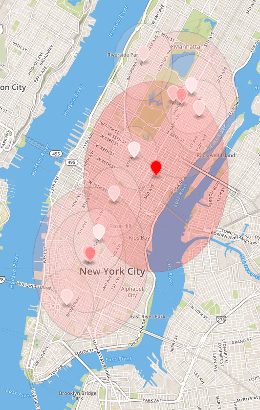
The vertical skew in circles comes from treating longitude and longitude equally for the radius. Unfortunately, the standard deviation is high. Big zones around markers indicate that often high-tip rides started far from the center of a cluster they belong to. Nonetheless, the clustering results appear to be satisfactory because they address the issue of finding areas with high tip.
Some adjustments could be made to obtain different clusters and better Silhouette scores. Most notably, the number of clusters could be changed. Also, the impact of the tip could be controlled with the setMax() method of the MinMaxScaler. Decreasing the maximal tip value would put more weight on the latitude and longitude, decreasing the geographical variance (at the cost of a bigger tip variance within a cluster).
Saving K-means models for each hour
Let’s compute 24 independent k-means models, one for each hour of the day. In place of the 10 am example, loop all hours while saving trained models to “kmeans-models” directory:
val k = 12
val startingHour = 0
val endingHour = 24
for (h <- startingHour until endingHour) {
    val pipeline = prepareKmeansPipeline(k)
    val datasetHour = dfRidesManhattan.filter(col("startHour") === h)
    val kmeansPipe = pipeline.fit(datasetHour) // obtain a PipelineModel
    //save with MLWriter
    kmeansPipe.write.overwrite.save(s"kmeans-models/clusters-at-$h")
}
Notice that the code to train the k-means models doesn’t involve calling computeVariances or generateGeoJSON functions.
Integration of the ML model within the streaming pipeline
The streaming data pipeline developed in the previous parts of this 4 articles series breaks down to:
- Streaming data is produced to Kafka
- Spark application consumes Kafka messages
- Kafka messages are parsed and converted into Spark DataFrames
- Raw dataset is persisted on HDFS
- Spark Structured Streaming processes the streaming data: cleaning, joining, feature engineering, and aggregating
- Results of the Spark processing are persisted in HDFS and stored in-memory
- Streaming results are exposed via JDBC for low-latency queries
The existing data pipeline will be modified to account for the inclusion of the Machine Learning algorithm. Mainly, the previous stream processing carried out by Spark Structured Streaming engine will be altered.
Create a “MainConsoleClustering.scala” file in the com.adaltas.taxistreaming package. Spark streaming application must have all the k-means models loaded:
import org.apache.spark.ml.PipelineModel
import org.apache.spark.ml.clustering.KMeansModel
// Read clusters in MainConsoleClustering
var hourlyClusters: Array[Array[org.apache.spark.ml.linalg.Vector]] = Array()
val startingHour = 0
val endingHour = 24
for (h <- startingHour until endingHour) {
    val reloadedKmeansPipe: PipelineModel = PipelineModel
    	.load(s"kmeans-models/clusters-at-$h")
    val centers: Array[org.apache.spark.ml.linalg.Vector] = reloadedKmeansPipe
    	.stages(2)
    	.asInstanceOf[KMeansModel]
    	.clusterCenters
    hourlyClusters = hourlyClusters :+ centers
}
Whenever an ending Taxi ride event will arrive from the stream, its ending hour will determine which of the 24 clustering models available via the hourlyClusters variable will be used. Still, hourlyClusters is an array of clusters (Vectors) - which cluster is the best recommendation for the free driver?
To find the best cluster for a driver, we will be comparing distances between clusters’ centers and the geographical coordinates of the finished ride. Define a function which allows to compute distance in meters between 2 geographical points:
def distBetween(lon1: Double, lat1: Double, lon2: Double, lat2: Double): Double = {
    // Distance between (lon1, lat1) and (lon2, lat2) in meters
    val earthRadius = 6371000 //meters
    val dLon = Math.toRadians(lon2 - lon1)
    val dLat = Math.toRadians(lat2 - lat1)
    val a = Math.sin(dLat / 2) * Math.sin(dLat / 2) +
    	Math.cos(Math.toRadians(lat1)) * Math.cos(Math.toRadians(lat2)) *
    	Math.sin(dLon / 2) * Math.sin(dLon / 2)
    val c = 2 * Math.atan2(Math.sqrt(a), Math.sqrt(1 - a))
    val dist = (earthRadius * c).toFloat
    dist
}
Next, let’s put the distBetween function to use inside a UDF function picking up an attractive cluster for the Taxi driver:
val RecommendedLonLat = udf { (h: Int, lon: Double, lat: Double) => {
    val clustersArray = hourlyClusters(h)
    var closestCluster = clustersArray(0) // Init to 1st cluster
    clustersArray foreach { case (vect) =>
        val clusterLon = vect(0)
        val clusterLat = vect(1)
        val clusterTip = vect(2)
        val dist = distBetween(clusterLon, clusterLat, lon, lat)
        val currentBestDist = distBetween(closestCluster(0),closestCluster(1),lon,lat)
        if ((dist < currentBestDist && (clusterTip > closestCluster(2))) {
            closestCluster = vect
        }
    }
    Seq(closestCluster(0), closestCluster(1))
}: Seq[Double] }
In the RecommendedLonLat function, all clusters from 1-hour time segment are scanned in order to match input point with closest cluster. To establish that a given cluster is better, not only it must be closer than the current best cluster, but also it would need to yield higher tip. Finally, geographical coordinates of the most appropriate clusters are exposed as recommended longitude and latitude.
The remaining code reflects the existing pipeline developed in the previous parts of the series. It mostly copies the content of the “MainConsole.scala” file.
import com.adaltas.taxistreaming.processing.TaxiProcessing
import com.adaltas.taxistreaming.utils.{ParseKafkaMessage, StreamingDataFrameWriter}

val taxiRidesSchema = StructType(Array(
    StructField("rideId", LongType), StructField("isStart", StringType),
    StructField("endTime", TimestampType), StructField("startTime", TimestampType),
    StructField("startLon", FloatType), StructField("startLat", FloatType),
    StructField("endLon", FloatType), StructField("endLat", FloatType),
    StructField("passengerCnt", ShortType), StructField("taxiId", LongType),
    StructField("driverId", LongType)))

val taxiFaresSchema = StructType(Seq(
    StructField("rideId", LongType), StructField("taxiId", LongType),
    StructField("driverId", LongType), StructField("startTime", TimestampType),
    StructField("paymentType", StringType), StructField("tip", FloatType),
    StructField("tolls", FloatType), StructField("totalFare", FloatType)))

// Adjust kafka "master02.cluster:6667" <-> "localhost:9997" (hadoop setup vs local)
var sdfRides = spark.readStream.
    format("kafka").
    option("kafka.bootstrap.servers", "master02.cluster:6667").
    option("subscribe", "taxirides").
    option("startingOffsets", "latest").
    load().
    selectExpr("CAST(value AS STRING)")

var sdfFares= spark.readStream.
    format("kafka").
    option("kafka.bootstrap.servers", "master02.cluster:6667").
    option("subscribe", "taxifares").
    option("startingOffsets", "latest").
    load().
    selectExpr("CAST(value AS STRING)")

sdfRides = ParseKafkaMessage.parseDataFromKafkaMessage(sdfRides, taxiRidesSchema)
sdfFares= ParseKafkaMessage.parseDataFromKafkaMessage(sdfFares, taxiFaresSchema)
sdfRides = TaxiProcessing.cleanRidesOutsideNYC(sdfRides)
sdfRides = TaxiProcessing.removeUnfinishedRides(sdfRides)
val sdf = sdfRides.withColumn("hour", hour(col("endTime")))
Finally, we can integrate a streaming data pipeline with the k-means models via the RecommendedLonLat UDF and output the results.
val sdfRes = sdf
    .withColumn("RecommendedLonLat", RecommendedLonLat(
        col("hour"), col("endLon"), col("endLat")))
    .drop(col("passengerCnt"))

// Write streaming results in console
StreamingDataFrameWriter.StreamingDataFrameConsoleWriter(sdfRes, "TipsInConsole").awaitTermination()
The Scala Spark application jar can be compiled with sbt-console, and submitted with spark-submit. In case of running on the Hadoop cluster from part 2 of the series, submit it with:
spark-submit \
  --master yarn --deploy-mode client \
  --class com.adaltas.taxistreaming.MainConsoleClustering \
  --num-executors 2 --executor-cores 1 \
  --executor-memory 5g --driver-memory 4g \
  --packages org.apache.spark:spark-sql-kafka-0-10_2.11:2.3.0 \
  /vagrant/taxi-streaming-scala_2.11-0.1.0-SNAPSHOT.jar
Otherwise, replace master with local and match your machine’s resources.
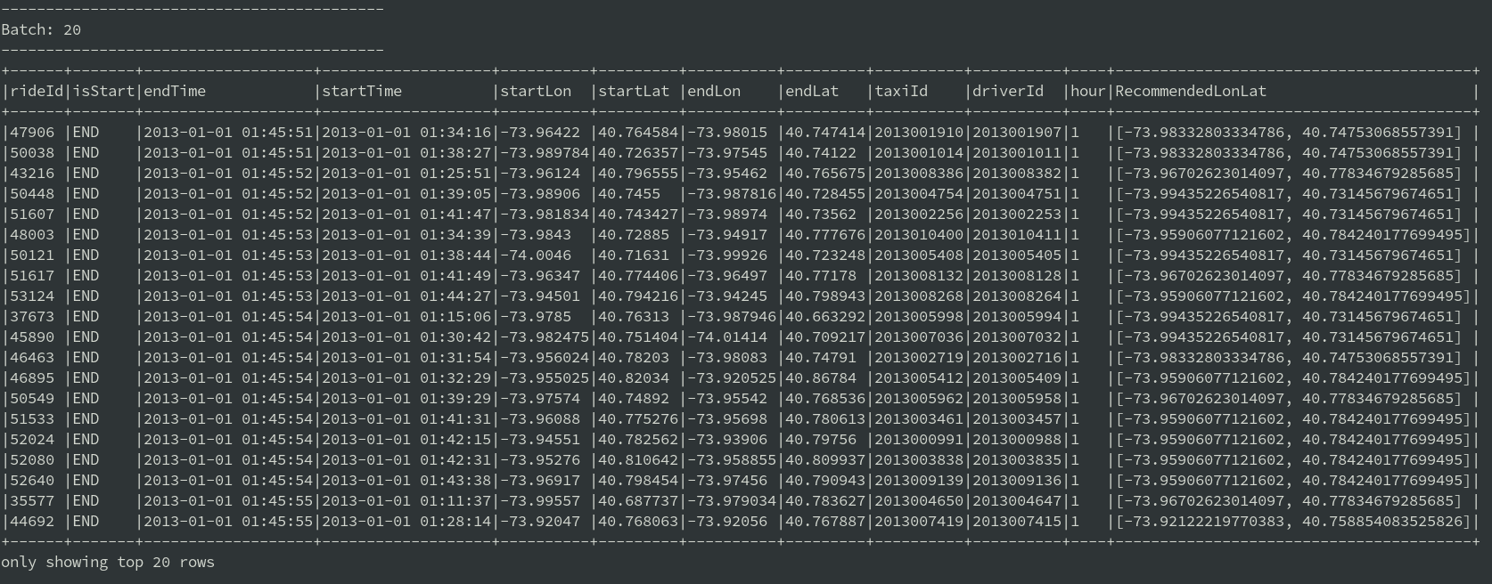
After launching Kafka streams (as explained in part 1 and 2 of the series), final results are written to the console:
Note that periodical updates of k-means models would need to be done on a Hadoop cluster. This could be achieved e.g. with Apache Airflow submitting Spark job with MainKmeans application. For example, each night clusters could be recomputed based on data from last week.
Conclusions
Most of the work in an ML project comes down to data preparation, preprocessing, understanding of the algorithm, and evaluation. This article reflects this, as a lot of work had to be done besides simply fitting Spark’s k-means algorithm on data.
Deployment of an ML model in a real-time scenario is generally difficult, but as shown in this article, this could be simplified. The k-means clustering, although training on static data, was successfully incorporated within a streaming data pipeline.
