Faster model development with H2O AutoML and Flow

Building Machine Learning (ML) models is a time-consuming process. It requires expertise in statistics, ML algorithms, and programming. On top of that, it also requires the ability to translate a business problem into mathematical formulas. The whole process consists of many steps. For example, when we receive a new dataset, we want to explore it first - decide which columns might be useful depending on the business question, handle missing values, check for the correlations, distributions, or the number of classes of the variables. Then we can finally decide which models will be the most appropriate and test their baseline performance. To improve the performance and get the most out of a model, we also need to tune the hyper-parameters and select the most appropriate metric for the question at hand. Coding and running these steps sequentially eats away the time that could otherwise be invested in a better understanding of the user story.

In order to bridge these problems, many frameworks emerged that automate at least some of them. They reduce the time required for human intervention and increase the number of automatically tested models or generated features. They are known as AutoML (Automatic / Automated Machine Learning). We are about to discover one of them, the open source H2O platform, through Python API and Flow, the Web UI.

Introduction to AutoML and H2O

Automatic Machine Learning (AutoML) is an approach to ML, where individual tasks are automated. These tasks could be:

• data pre-processing
• feature engineering, extraction, and selection
• testing many models from different families
• hyper-parameter optimization.

The goal of AutoML is different when applied to a Deep Learning or a Machine Learning context:

• Deep Learning for images, videos, and text data: trying to decipher the neural network architecture
• Machine Learning for tabular data: find the best model with the least amount of effort.

In this article, we will look into the second example. Open-source H2O helps us mostly with modeling and hyper-parameter tuning and to some extend with data pre-processing (e.g. imputation of missing values). To automate feature engineering, the H2O.ai company developed DriverlessAI, which is a proprietary product with a 21 day free trial available.

H2O is an open-source in-memory prediction engine which supports distributed computing. It can run on your laptop or on big multi-node clusters, in your on-premises Hadoop cluster as well as in the cloud. It is not limited by cluster size. Thus, you can handle big datasets and compute models in parallel. When working on an H2O cluster, the data is distributed over the nodes. The core algorithms are written in Java. The APIs are available for Python, R, Scala, and H2O Flow, their web-based interface. There is also a version that can be used with Spark, called Sparkling Water. Native connectors to different data storage facilitate the data import (local file system, remote files through URL, S3, HDFS, JDBC, and Hive) and several different file formats are supported (Parquet, Avro, ORC, CSV, XLS/XLSX, ARFF, and SVMLight).

We can choose among many different supervised and unsupervised algorithms:

• unsupervised: Aggregator, Generalized Low Rank Models, Isolation Forest, K-Means Clustering, and Principal Component Analysis.
• supervised: Cox Proportional Hazards, Deep Learning, Distributed Random Forest, Generalized Linear Model, Generalized additive models, Gradient Boosting Machine, Naive Bayes Classifier, RuleFit, and Support Vector Machine. We can optimize them in a ‘classical’ way one-by-one, or we can use the AutoML function, which will build many models during each experiment. We can also build Stacked Ensembles, where we combine multiple models into a better performing ‘metalearner’.

Once a model is built and verified, we can download it as a Java object. It can then be deployed to any Java environment.

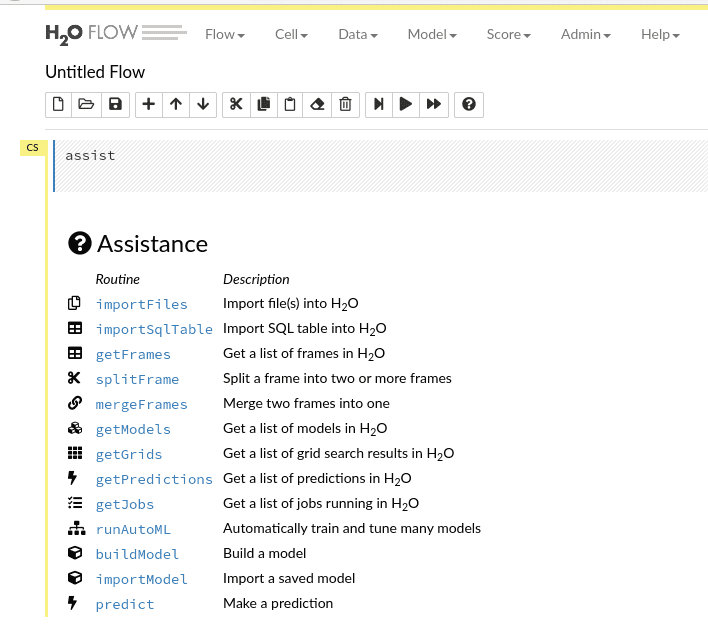
H2O Flow is a notebook-based Web UI in which we can point-and-click through the entire ML workflow. Each clicked automatically generates CoffeeScript code. These materialized clicks permit us to save the exact steps of the process (called Flow) and facilitate sharing and reproducibility. Flow has very limited functionalities for data preparation and feature engineering. Its power becomes evident in the modeling phase. When we click through the workflow, it exposes all the parameters of the methods and algorithms with a short description. Since the parameters are numerous, this is much faster than reading documentation, especially for less experienced Data Scientists or Analysts. It automatically creates a vast amount of plots, from partial correlation plots, AUC, gains/lift charts to variable importance and we can walk through them effortlessly. All this significantly decreases the time and the efforts spent on visualization and also increases the understanding of the studied model.

Moreover, we don’t need to choose between the versatility of an API and the user-friendliness of Flow. They can be used in conjunction to benefit from the best of both worlds. We will work on an example where we will prepare the data in Jupyter Notebook and save it. Then, we will import it in Flow and go through the next steps: parsing and modeling with AutoML, prediction, and, for the end, looking at the performance plots. This is a basic but common usage, where we minimize the coding and maximize the use of the GUI. More experienced Data Scientists will prefer to define and to starte the modeling phase programmatically and use Flow to visualize the progress and the results.

Environment setup

Pre-requisites are Java and web browser. I am currently using Arch Linux with Java 13 OpenJDK, Firefox 78.0.2, H2O 3.30.0.7, and Python 3.7.7.

Installation of Flow

To be able to run Flow on your computer, you need to install the latest stable release of H2O. Unzip the file, go to the unzipped directory and run h2o.jar:

cd h2o-3.30.0.7
java -jar h2o.jar

H2O is by default using port 54321. Therefore, when H2O starts, go to the web browser and open Flow by pointing to http://localhost:54321. Flow uses its own terminology and mode of functioning. You can familiarize yourself with it on the project documentation.

Installation of H2O for Python

I was using Miniconda, version 4.8.3.

Create a virtual environment:

$ conda create --name env_h2o python=3.7
$ conda activate env_h2o

Install the dependencies:

pip install requests
pip install tabulate
pip install "colorama>=0.3.8"
pip install future

Install the latest stable version of H2O:

pip install http://h2o-release.s3.amazonaws.com/h2o/rel-zahradnik/7/Python/h2o-3.30.0.7-py2.py3-none-any.whl

Dataset

The datasets used in this demo are client_train.csv and invoice_train.csv of Fraud Detection in Electricity and Gas Consumption.

Data pre-processing with Python API

The pre-processing part of our dataset was done in a jupyter notebook.

Initialize the H2O cluster

# start the H2O cluster
import h2o
h2o.init()

This starts the H2O cluster and gives us some details about its configuration: free memory, number of total and allowed cores, and on which URL we can access Flow. Here we are initializing the cluster with default parameters. They are a lot of them and they can be changed.

Import the dataset

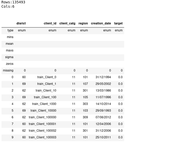
Note that H2O separates between file upload (data are pushed from the client to the server) and import (pulls the data that is already present on the server). Since we are running an H2O server on a local computer, both methods behave the same. We will import files with defined column types to do fewer conversions later on.

client_types = ['enum', 'enum', 'enum', 'enum', 'enum', 'enum']
client = h2o.import_file("../h2o/data/client_train.csv", col_types=client_types)
client.describe()

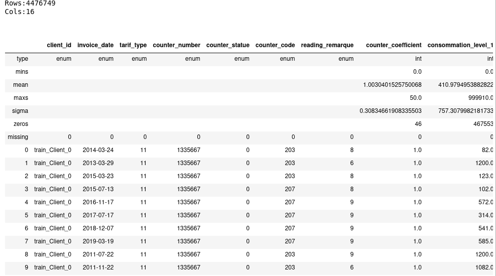
invoice_types = ['enum', 'enum', 'enum', 'enum', 'enum', 'enum', 'enum', 'int', 'int', 'int', 'int', 'int', 'enum', 'enum', 'enum', 'enum']
invoice = h2o.import_file("../h2o/data/invoice_train.csv", col_types=invoice_types)
invoice.describe()

Data pre-preprocessing

• Merge client and invoice tables: H2O implements two efficient merging methods (radix and hash method), which allow fast merging even when we have big data frames. However, columns used to merge them cannot be of the type string.

client_invoice = invoice.merge(client)

• Change date columns to time format: H2O automatically recognizes two different date formats during file parsing (yyyy-MM-dd and dd-MMM-yy). You need to convert others by yourself.

client_invoice['creation_time'] = client_invoice['creation_date'].as_date('%d/%m/%Y')
client_invoice['invoice_time'] = client_invoice['invoice_date'].as_date('%Y-%m-%d')

• Rename the columns disrict and counter_statue:

client_invoice.rename(columns={'disrict':'district', 'counter_statue':'counter_status'})

• Impute missing values with mode:

client_invoice.impute("counter_status", method="mode")

• Feature engineering: create a new column indicating how long someone is a client when receiving the invoice. We will delete all the clients where the billing date was before the creation date.

client_invoice['fidelity_period'] = client_invoice['invoice_time'] - client_invoice['creation_time']
client_invoice['total_consommation'] = sum(client_invoice[8:11])
client_invoice = client_invoice[client_invoice["fidelity_period"] > 0,  :]

• Save the data. We finished with the data pre-processing. If we want to use it with Flow, we need to persist it and import it in Flow.

h2o.export_file(client_invoice,"../h2o/data/client_invoice_1.csv")

In this short exercise, we saw several methods for data preparation, native to H2O, and working on distributed H2O frames. H2O covers a large range of methods but many others are not (yet) implemented. In these cases, we can use other libraries like Pandas and scikit-learn. We can easily transform the H2O frame to Pandas, but we need to keep in mind that the latter is not distributed.

Modeling with Flow

Open Flow on http://localhost:54321.

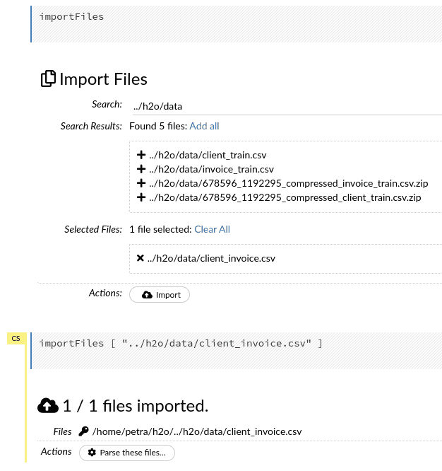
Import the data

If you type the path of the folder with your data and press “Enter”, you will obtain a list of all files in the folder. You can select one or more if your data is stored in a distributed format.

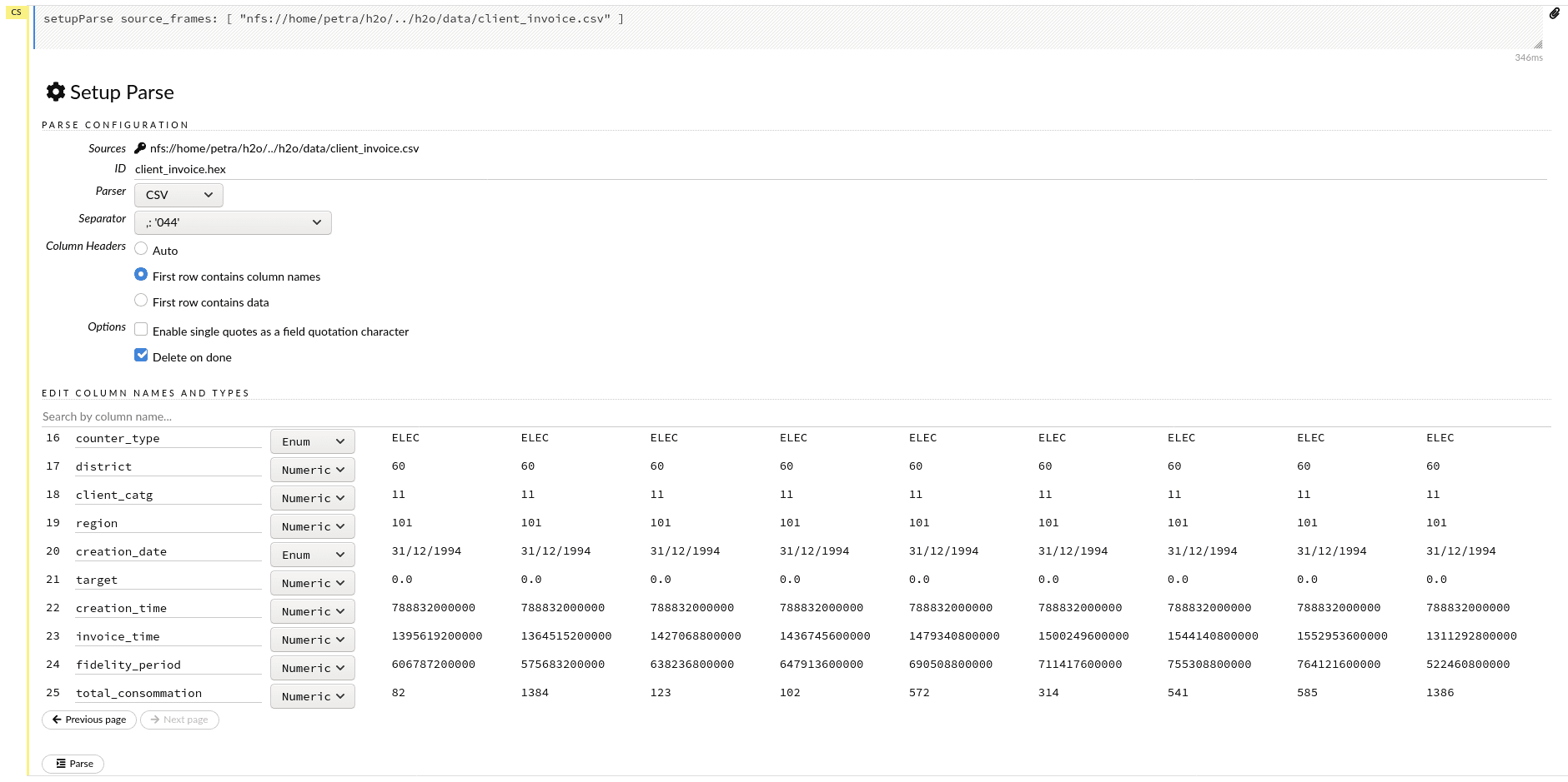
Parse

At import, the schema is automatically inferred. If we are not satisfied with the recognized data types in the columns, or with the separator and header that the parser chose, we can easily change them with the help of drop-down menus and radio buttons.

Below is the schema of the client_invoice data frame that we will be using, so let’s modify what’s needed. Here you can see that with datasets with many columns this becomes a very tedious task.

{'client_id': 'Enum',
 'invoice_date': 'Enum',
 'tarif_type': 'Enum',
 'counter_number': 'Enum',
 'counter_status': 'Enum',
 'counter_code': 'Enum',
 'reading_remarque': 'Enum',
 'counter_coefficient': 'Numeric',
 'consommation_level_1': 'Numeric',
 'consommation_level_2': 'Numeric',
 'consommation_level_3': 'Numeric',
 'consommation_level_4': 'Numeric',
 'old_index': 'Enum',
 'new_index': 'Enum',
 'months_number': 'Enum',
 'counter_type': 'Enum',
 'district': 'Enum',
 'client_catg': 'Enum',
 'region': 'Enum',
 'creation_date': 'Enum',
 'target': 'Enum',
 'creation_time': 'Numeric',
 'invoice_time': 'Numeric',
 'fidelity_period': 'Numeric',
 'total_consommation': 'Numeric'}

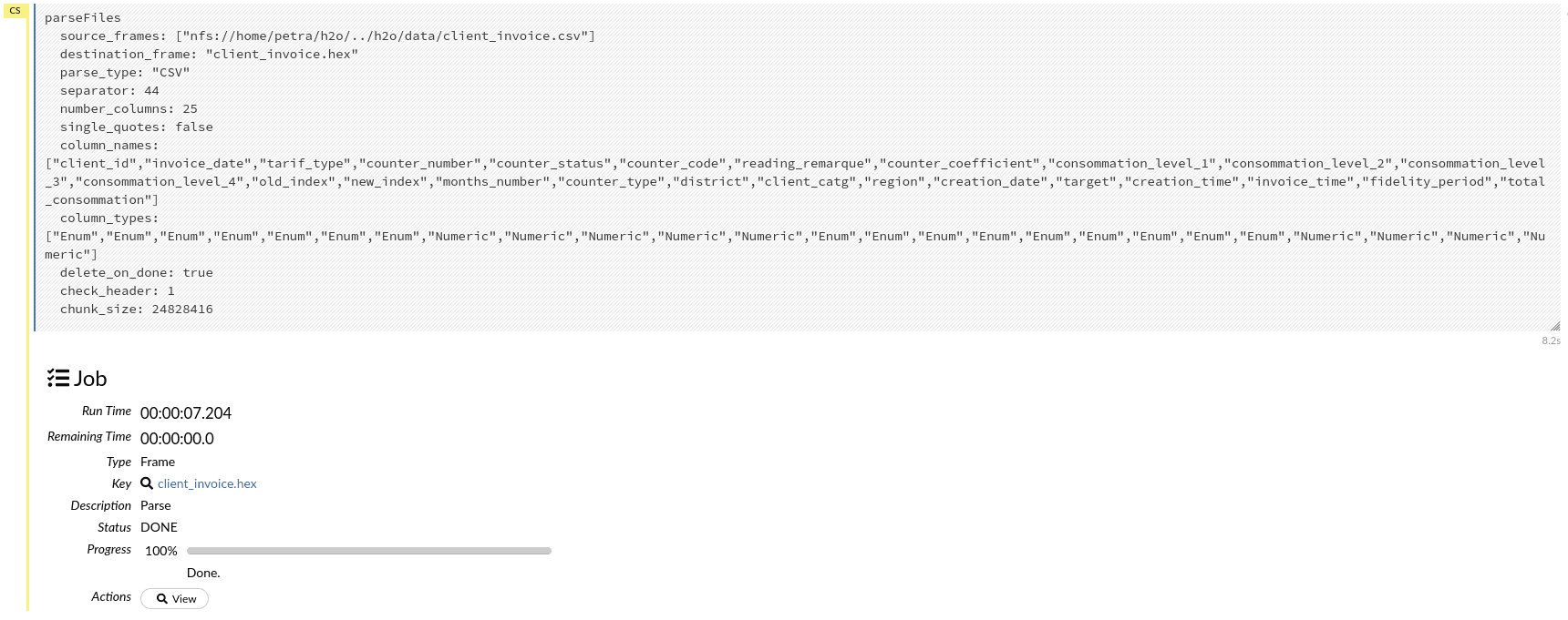
Clicking on Parse will start the parsing.

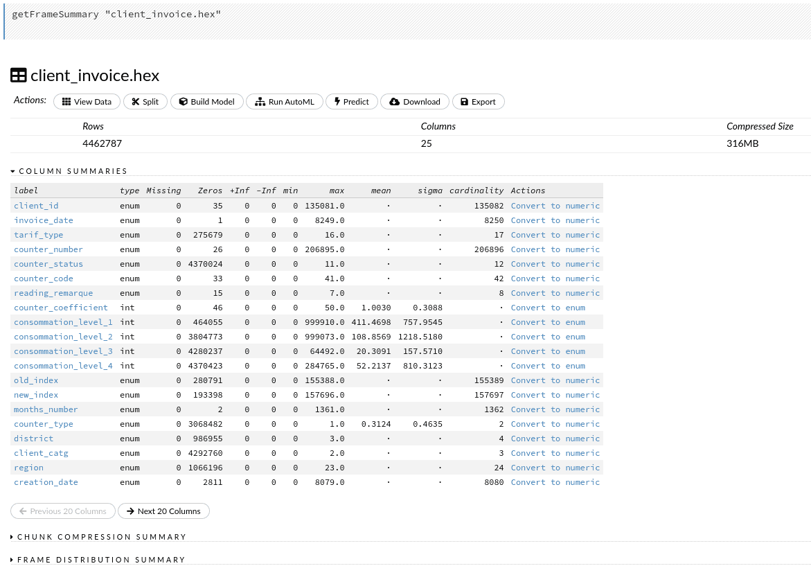
The next action we can do is View. We can re-inspect the table again, this time with summary statistics of all columns. If we compare it with .describe() output from the notebook, we can appreciate the added information about the cardinality of categorical variables.

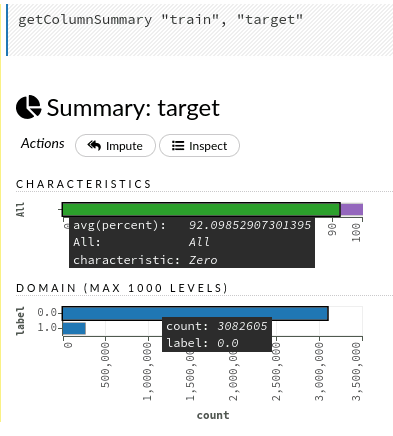
If we click on the name of a column, we will discover even more details about each column. Let’s try with the response variable target. Clicking on the name opens plots with the ratio of zeros vs. other values and distribution of labels. Inspect above the plots leads us to the raw data used to create the two plots. Also, if we wouldn’t impute the missing values before, we could do it in this step.

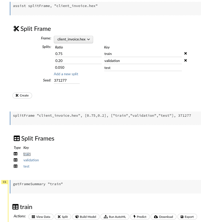
Split

Now we will split the data into train, validation and test sets (75%, 20%, 5% respectively). Create the frames and click on train to generate the list of actions.

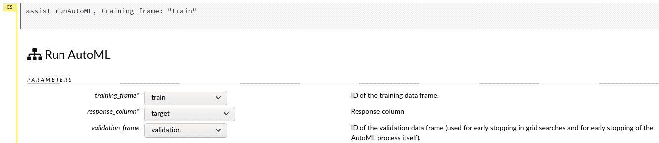
Run AutoML

We reached the stage where we can Run AutoML. First, we need to select the training and the validation data frame and specify the response variable.

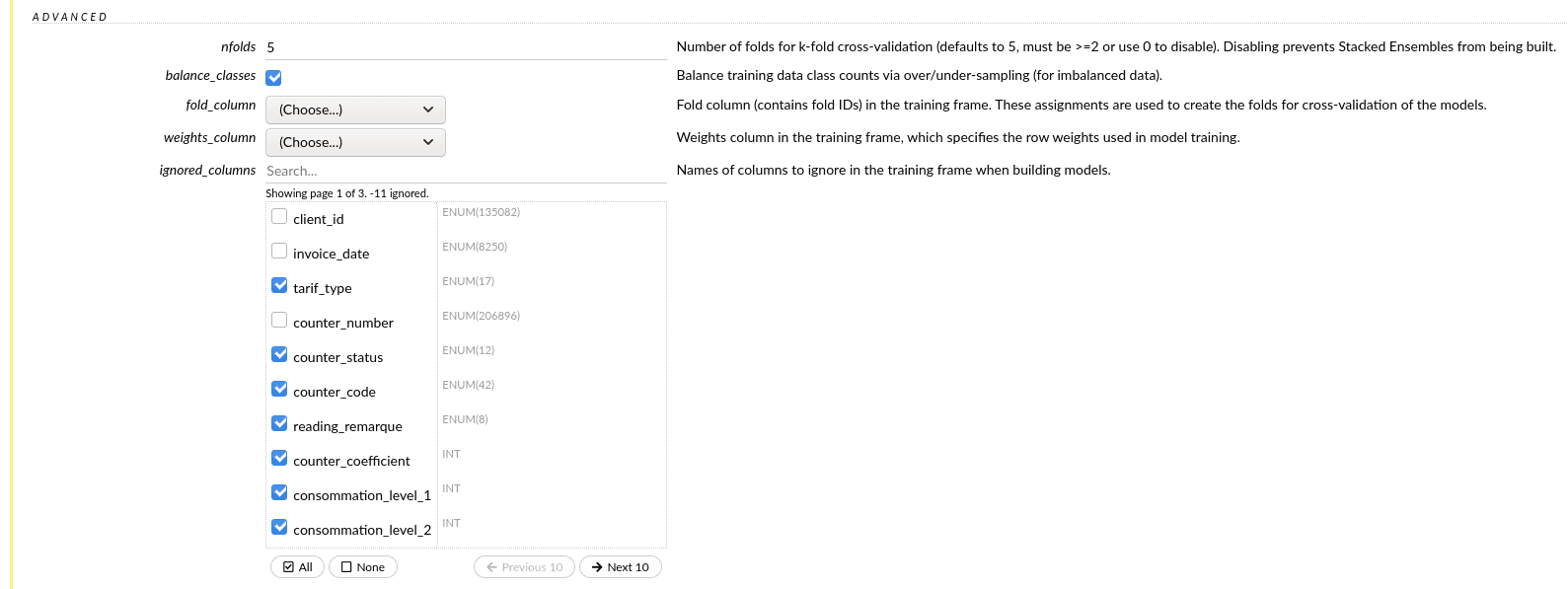
Then, we need to tick the columns we want to exclude from modeling. We want to keep the following ones:

['tarif_type', 'counter_status', 'counter_code', 'reading_remarque', 'counter_coefficient', 'consommation_level_1', 'consommation_level_2', 'consommation_level_3', 'consommation_level_4', 'counter_type', 'district', 'client_catg', 'fidelity_period', 'total_consommation']

Since frauds are rare events, the datasets for fraud prediction tend to be strongly unbalanced. In our case 7.9% of instances represent frauds. We will use balance_classes option, which will help us to handle this issue.

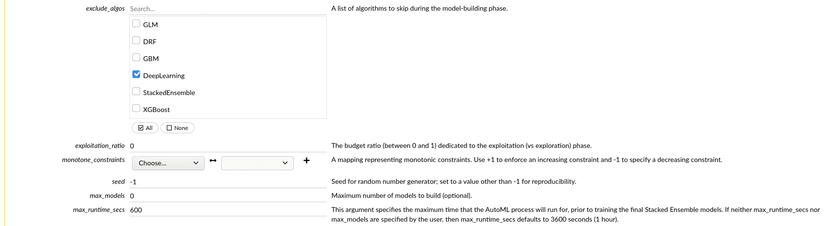
We can exclude the algorithms we are not interested in. To illustrate, let’s exclude Deep learning. We will also specify the time the AutoML should run before starting to build stacked models. I set it to 600 seconds, and the total runtime was 14.5 minutes, including building two stacked models at the end.

When we set up all the parameters, we click Build models.

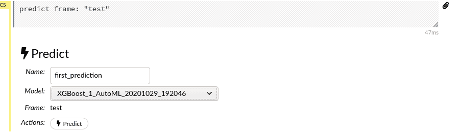
Prediction

Now that the models are trained and validated, we can test them on our test dataset. We need to go back to our Split Frames and select the test frame. On the action list we select Predict and from the drop-down menu Model the model we would like to use.

Metrics and Plots

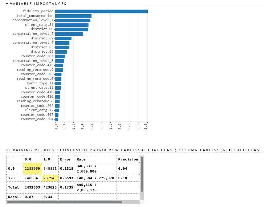
To explore in detail the performance of a model, we click on its name in the leaderboard after an AutoML run, or we can get the list of all of the models in our environment with the function getModels. Here we can find visualizations of different metrics (logloss, auc), variable importance plot, confusion matrices, gain/lift tables, list of model parameters, cross-validation reports, etc.

Export of Models

You can export your favorite model as a Java code and run it on whichever Java environment. This reduces the need for translating the model from Python or R code into a language used in production and risk potential implementation errors. Also, like a Java object, the model is decoupled from H2O environment.

Conclusion

In this tutorial, we saw a fast and effortless way of building models with H2O. In addition, the framework gives us information about model performance and feature importance, which helps us understand and interpret the models. It trains several tens of models using n-fold cross-validation in a matter of hours or days, depending on the size of the dataset and the quality of the training you wish. It can answer several important questions like ‘What model family works the best?’ and ‘Which are the most important variables?‘. It provides us good starting values for the model parameters, which we can further optimize. But to squeeze out the best possible performance, H2O open-source is not enough and we invite you to look at the product propose by H2O.ai, the company behind the open source project. For example, automated hyper-parameter tuning is quite basic and it lacks the optimized grid search. Also, the data needs to be prepared elsewhere. Nevertheless, it speeds up significantly the initial stages of modeling and reduces the amount of the code we need to write, so we invest more time in understanding the underlying use cases.

References:

• H2O official website
• Automatic Machine Learning with H2O AutoML (video)
• Applying Machine Learning Using H2O (video)
• Erin LeDell - Scalable Automatic Machine Learning with H2O (video)
• H2O - Hands-on with R, Python and Flow with Amy Wang (video)